Finding the joins your warehouse never declared

Statistical foreign-key inference, validated against real data. How ktx builds the join graph agents rely on.

Part 2 of 6. Building a context layer for data agents.

The missing join graph

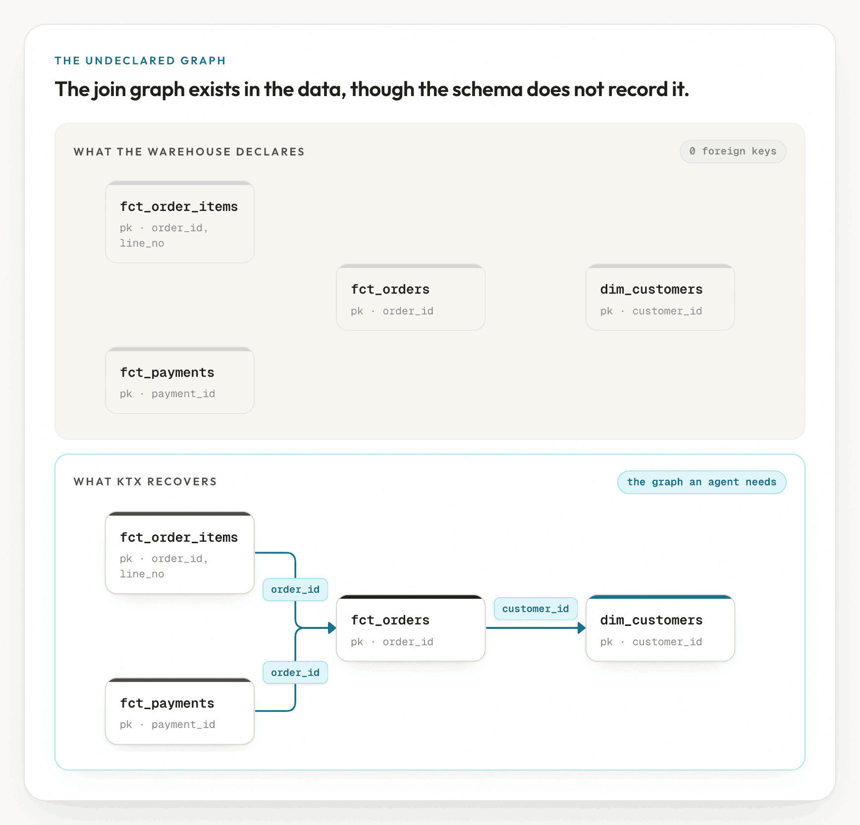
Open the information schema of almost any analytics warehouse and look for foreign keys. A transactional Postgres instance may declare a few. A BigQuery or Snowflake warehouse fed by ELT usually declares none.

The loader that built fct_orders never declared that customer_id references dim_customers.customer_id. The warehouse does not enforce the constraint in any case, and declaring it only slows loads. The relationship therefore survives only informally: in an analyst's memory, in a dbt relationships test when one exists, and in the many ad-hoc queries that each rediscovered it.

This missing graph is precisely what an agent requires and cannot obtain. In Part 1 we examined what happens when a text-to-SQL agent infers a join incorrectly: it expands a one-to-many relationship, double-counts the measure, and returns a revenue figure that is silently inflated.

The error was not arithmetic but a modeling error: the agent joined two tables on columns that do not form a key relationship, or it selected the wrong parent for an ambiguous id column. The query executed successfully and returned an incorrect result, with no error raised.

The question that Part 1 leaves open is the one this post addresses: where does a trustworthy join graph come from when the warehouse never declared one?

Three straightforward answers each fail:

• Reading the graph off the schema is impossible, because the schema does not record it.
• Trusting the column names is unreliable, because account_id is a free-text external reference in one table and a genuine key in another.
• Asking a human to hand-model every join in a five-hundred-table warehouse before the agent may run is impractical.

The graph must instead be recovered: inferred, then each inference proven against the data before an agent relies on it for a query.

The general technique: infer, score, then verify

The discipline that recovers an undeclared join graph is statistical schema profiling and join inference, studied under names such as foreign-key discovery and inclusion-dependency mining.

The structure is consistent across these methods: generate candidate joins from inexpensive signals, score them, and then, in the step most in-house implementations omit, validate the surviving candidates against real data rather than trusting the signals that proposed them.

Each of the alternatives is a choice that some team makes, and each fails in a characteristic way.

Trusting declared foreign keys only. This is clean but yields the empty graph described above. On a modern ELT warehouse the strategy finds almost nothing, because almost nothing is declared.

Naming-convention heuristics. "Any column ending in _id joins to the table whose name it carries." This is fast and correct often enough to be misleading. It proposes orders.user_id → users.id when users was deprecated two migrations ago and the live values point at app_users. Names suggest joins but do not prove them.

Manual modeling. A dbt project with relationships tests, or a hand-built LookML model, encodes joins a human verified. This is the most reliable option for the joins someone has modeled, but it leaves the remaining majority uncovered. It also becomes stale, without warning, as soon as a loader adds a column.

BI-tool relationship editors. Looker, Metabase, and similar tools allow relationships to be drawn in a UI. The trade-off matches manual modeling, with the additional limitation that the graph is confined to one tool's metadata rather than stored alongside the data.

The common lesson across all four is that a name, a type, or a convention is a hypothesis, not a fact. The only operation that converts "these columns are named like a key relationship" into "these columns are a key relationship" is checking whether the child values actually appear in the parent.

Coverage and violation counts are the ground truth. Everything upstream of them is a means of deciding which hypotheses justify the cost of a verification query.

This cost is the reason for the funnel. In principle, every column pair in the warehouse could be validated, but that requires one verification query per pair. The cost is quadratic in the number of columns, which is both slow and a heavy load on the warehouse.

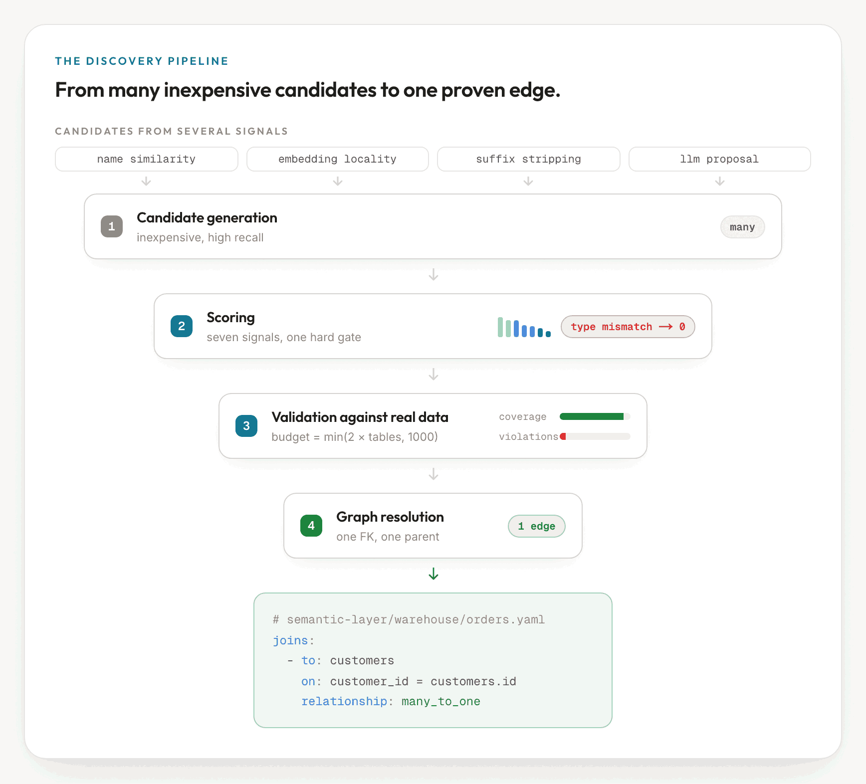
The technique is therefore a narrowing pipeline: many inexpensive candidates in, a scored shortlist, a budgeted set of real-data checks, and a resolved graph out. The remainder of this post describes how ktx builds that pipeline.

The discovery pipeline in ktx

In ktx, recovering the join graph is one stage of the database scan, the stage the context engine relies on later when it compiles a metric into safe SQL. The stage runs in a fixed order and begins by profiling every reachable column for uniqueness, null rates, and a sample of values. Profiling is what converts names into evidence: a column named id that is also unique and non-null is a far stronger key candidate than one that merely appears to be a key.

Generating candidates from several signals

Candidate generation is deliberately high-recall, because proposing a spurious join that validation later rejects is cheaper than missing a real one. Four independent signals feed it, so that a join one signal misses, another may still catch.

• Suffix stripping turns customer_id into customer and matches it to a customers table.
• Name similarity ranks which tables are worth considering as parents, so that scoring never runs on every column-and-table pair.
• Embedding locality catches synonyms such as buyer and customer that share no name tokens.
• LLM proposals are optional and outside the critical path: a model may suggest likely keys, but those suggestions undergo the same scoring and validation as every other candidate. The model can propose candidates but does not decide which are accepted.

Anything that merely restates a foreign key the warehouse already declares is discarded.

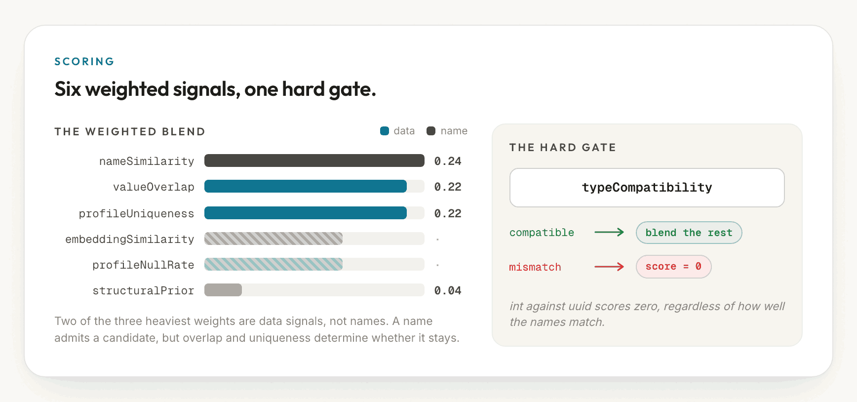
Scoring: seven signals and one hard gate

Every surviving candidate receives a confidence score that blends seven signals, each guarding a different failure mode (below). The most heavily weighted are nameSimilarity, valueOverlap, and profileUniqueness, and two of those three are data signals rather than name signals: a name admits a candidate, but overlap and uniqueness determine whether it remains.

One signal is not a weight at all. typeCompatibility is a hard gate: if the two column types cannot join, the score is zero regardless of how well the names match. It remains lenient toward genuine equivalents (int4 with bigint, varchar with text), but a mismatch across type families is disqualifying. This single rule eliminates a whole class of plausible-looking false positives before any of them incurs a query.

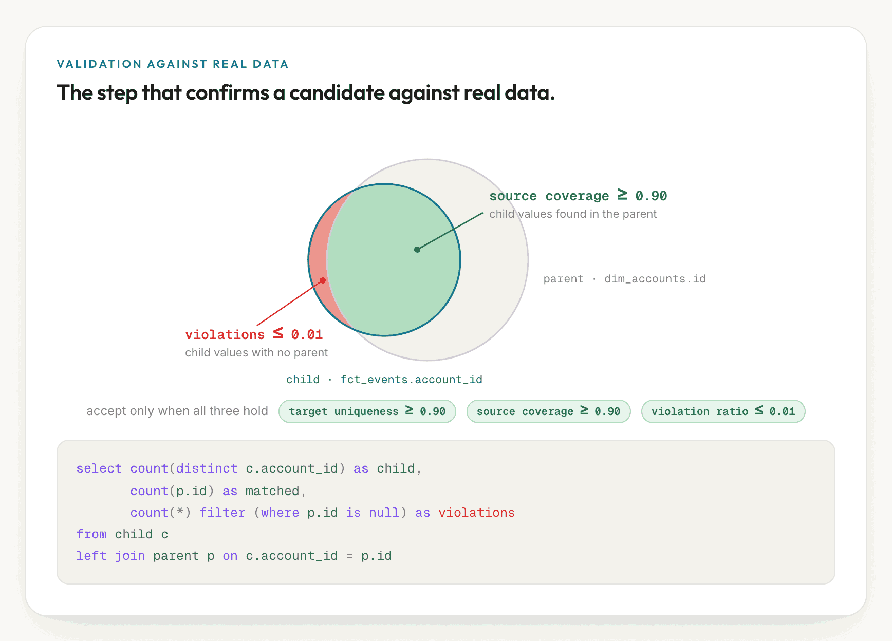
Validating against real data

Scoring ranks candidates but does not confirm them. Confirmation requires a SQL query. For each candidate that clears the budget, the engine collects the distinct values of the child column and of the parent, left-joins them, and counts how many child values have no matching parent.

The accept gate is strict and the thresholds are exact. Nearly all child values must match the parent (sourceCoverage at least 0.90, violationRatio at most 0.01), and the parent column must itself be near-unique (at least 0.90). If any one threshold is missed, the candidate is rejected outright, regardless of its name score. This is where the silent failures of the naming-convention approach are caught: a candidate that appears ideal but whose values point at a deprecated table covers nothing. A candidate that clears the gates is marked accepted. One that falls between the thresholds is marked review and is never accepted automatically.

A validation budget

Every validation is a real query against the warehouse, so the engine caps how many it runs at min(2 * tables, 1000) and validates candidates in confidence order. The remainder are deferred to review rather than dropped, so that a later run can complete them. The funnel narrows precisely so that the expensive step runs only on the candidates most likely to survive it.

Resolving the graph: one foreign key, one parent

Validation returns a set of edges, but a set of edges is not yet a graph. The resolver settles two questions. First, it establishes primary keys, because a foreign key is only as trustworthy as the key it references. Where none is declared, it reconstructs one from the profile: a column that is unique, non-null, and the target of validated references.

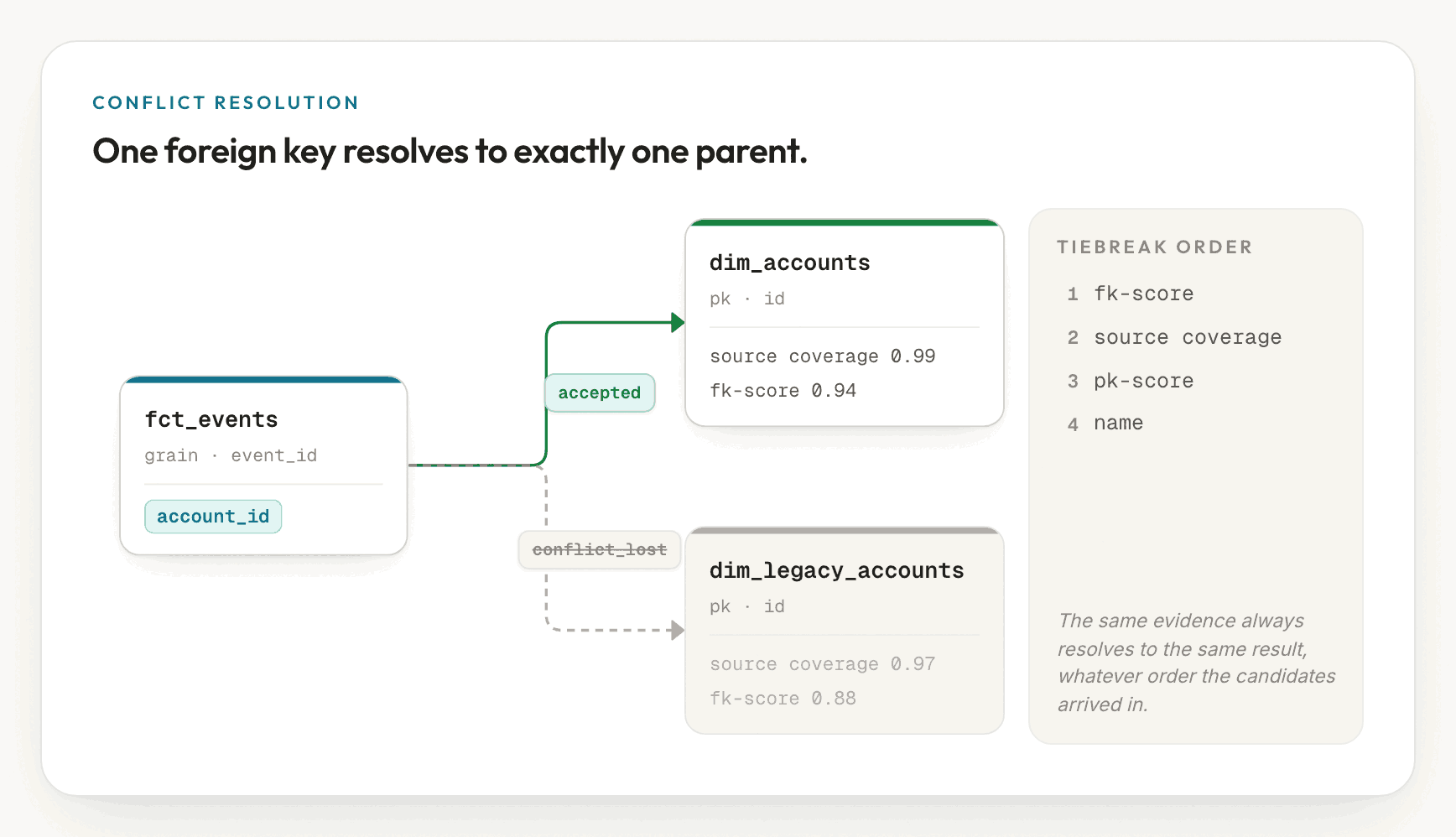
Second, and more importantly, it enforces that one foreign-key column references exactly one parent. When events.account_id validates against both accounts.id and legacy_accounts.id because the data overlaps, the resolver ranks the competing candidates by foreign-key score, then source coverage, then primary-key score, and finally a stable name comparison. The top edge stays accepted and the rest are demoted to conflict_lost. The outcome is one column to one parent, determined by a fixed rule rather than by whichever candidate happened to be scored first, consistent with the deterministic approach the ingestion engine takes elsewhere in ktx.

Composite keys: when a single column is not the key

A real join graph does not consist only of single-column keys. Bridge tables and event tables are often keyed on two or three columns together, such as (order_id, line_number). A separate pass tests column tuples for uniqueness and validates their coverage in the same way, holding them to the same strict thresholds as single-column joins.

Summary and takeaways

Setting aside the specific names and thresholds, the entire design reduces to a single principle: a join is a hypothesis until the data confirms it.

Names, types, embeddings, and even an LLM's reading of the schema are all merely means of deciding which hypotheses are inexpensive enough to test. The only operation that promotes a candidate to an accepted edge is a real query demonstrating that the child values occur in the parent.

For practitioners implementing a similar system, the transferable rules are as follows:

• Generate from several signals rather than one. Any single heuristic (names, types, or embeddings) has a blind spot. Overlapping signals raise recall before a verification query is spent.
• Treat type compatibility as a gate, not a weight. A type mismatch must be disqualifying, not merely discouraging. It is the least expensive way to eliminate a whole class of false positives.
• Validate against real data and reject on a hard threshold. Coverage and violation counts are the only ground truth. Choose explicit thresholds (ktx uses 0.90 coverage, 0.01 violations, and 0.90 target uniqueness) and reject anything that fails them, rather than allowing a high name score to compensate for thin data.
• Budget the verification. Real queries incur real cost and load. Rank by confidence, validate the top slice, and defer the remainder to review rather than overloading the warehouse or discarding candidates.
• Resolve to one parent per key, deterministically. A graph with ambiguous edges is worse than no graph, because an agent will select one edge and the choice will be opaque. A fixed ranking with stable tiebreakers ensures that the same set of competing candidates always resolves to the same result.

The result of ktx's specific choices is a join graph that an agent can rely on for a query without a human having pre-modeled every relationship. Every edge in the graph carries its own evidence: the coverage it cleared, the number of violations it incurred, and the competing edge it was ranked above for that column.

This evidence matters more than it may appear, because the graph is not the end of the process. It is the input to a compiler. The accepted edges become the join paths that Part 1's SQL compiler traverses when it compiles a metric into safe SQL, which is precisely why the graph must be correct, not merely plausible, before anything is permitted to join on it.

A recovered join graph is only one of several places where a data stack quietly disagrees with itself. The next is more conspicuous: when dbt, Looker, and Metabase each define "revenue" differently, one of the definitions is wrong, and the system must detect the disagreement rather than silently adopt one.

Part 2 of 6. Building a context layer for data agents.

Previous: Why your data agent keeps writing SQL that double-counts. Next in the series: when dbt, Looker, and Metabase disagree on "revenue".